What is a classification tree?
- Tree that predicts a categorical response using most commonly occuring class of leaf and chooses splits that minimize a different criterion (discussed below)
How to build a regression tree with Scikit Learn?
1.How to load data?
- Import usual libraries
import pandas as pd
import numpy as np
import matplotlib.pyplot as plt
%matplotlib inline
2. Use csv path as argument of pd.read_csv
pd.read_csv('/Users/omaraguilar/DSI_SM_01/curriculum/week-06/1.2-lab/assets/datasets/cars.csv')
3. Store result in a variable
df = pd.read_csv('/Users/omaraguilar/DSI_SM_01/curriculum/week-06/1.2-lab/assets/datasets/cars.csv')
df.head(10)

2. What is the essential data?
- Do we need to drop data? Sum NaN to find out
df.isnull().sum()

3. Is our essential data in the right format?
- We’ll solve that in Step 4
4. Choose data features and target
1. Define target (what we want to predict)
- No
- How express categorical values in a boolean way?
- target is acceptability
2. How to turn target into the right format?
- Import Label Encoder
from sklearn.preprocessing import LabelEncoder
- Instantiate encoder
le = LabelEncoder()
- Transform target column into boolean values by applying label encoder function to it
le.fit_transform(df['acceptability'])
- Store result in a variable that represents target
y = le.fit_transform(df['acceptability'])
3. Data features (everything but target and non-numeric columns)
- data features are non-acceptability
4. How to turn data features into the right format?
- Drop target column from data features setting axis parameter to numeric representation of vertical
df.drop('acceptability', axis =1)
- Use result as argument of pd.get_dummies
pd.get_dummies(df.drop('acceptability', axis=1))
- Store new result in a variable that represents data features
X = pd.get_dummies(df.drop('acceptability', axis=1))
4. Choose training and testing data
1. Use train_test_split method and data features as first argument, target as second argument and set test_size parameter to your desired percentage, and random_state parameter as whathever number you want
train_test_split(X, y, test_size=0.3, random_state=42)
2. Store method in four variables (X_train, X_test, Y_train, Y_test)
X_train, X_test, Y_train, Y_test = train_test_split(X, y, test_size=0.3, random_state=42)3. See your training data

5. Create tree classification model (this is the part where regression and classification tree differ)
1. Import class (DecisionTreeRegressor from sklearn.tree)
from sklearn.tree import DecisionTreeClassifier
2. Instantiate estimator specifying max_depth parameter if you want
treeclf = DecisionTreeClassifier(max_depth=3, random_state=1)
3. Fit training data to create model
treeclf.fit(X_train, y_train)
4. Predict predicted Y_test data using X_test
treeclf.predict(X_test)
(Step 6 through 10 are shown in Tree Classifier blog post)
11. Now, that you have improved your Regression Tree, determine importance of each data feature
- Create a dictionary whose keys are ‘feature’ and ‘importance
{'feature': 'importance': }2. Set ‘feature’s value to Data Feature columns and ‘importance’s value to method treeclf.feature_importances_
{'feature':X.columns,'importance':treeclf.feature_importances_}3. Use dictionary as data of Pandas DataFrame
pd.DataFrame({'feature':X.columns,'importance':treeclf.feature_importances_})
4. Order DataFrame’s importances in descending order applying .sort_values(‘importance’, ascending=False) to result above
pd.DataFrame({'feature':feature_cols,
'importance':treeclf.feature_importances_}).sort_values('importance',
ascending=False).head()
5. See output

12. How to visualize our Regression Tree as an actual mental tree instead of a X vs. y function?
- Install
pydot2andgraphviz
2. Import the following
from IPython.display import Image
from sklearn.tree import export_graphviz
from sklearn.externals.six import StringIO
import pydot
3. Write the following
dot_data = StringIO()
export_graphviz(treereg, out_file=dot_data,
                feature_names=X.columns,
                filled=True, rounded=True,
                special_characters=True)
graph = pydot.graph_from_dot_data(dot_data.getvalue())
Image(graph.create_png())

4. Interpret tree diagram
Internal nodes
samplesis the number of observations in that node before splittingmseis the mean squared error calculated by comparing the actual response values in that node against the mean response value in that node- First line is the condition used to split that node (go left if true, go right if false)
Leaves
samplesis the number of observations in that nodevalueis the mean response value in that nodemseis the mean squared error calculated by comparing the actual response values in that node against “value”
13. Compute confusion matrix
- Import confusion matrix
from sklearn.metrics import confusion_matrix
2. Write confusion_matrix function
confusion_matrix()
3. Use y_test (actual testing target) and treeclf.predict(X_test) (predicted testing target) as arguments of confusion matrix function
confusion_matrix(y_test, treeclf.predict(X_test))
4. Store result in a variable
conf = confusion_matrix(y_test, treeclf.predict(X_test))
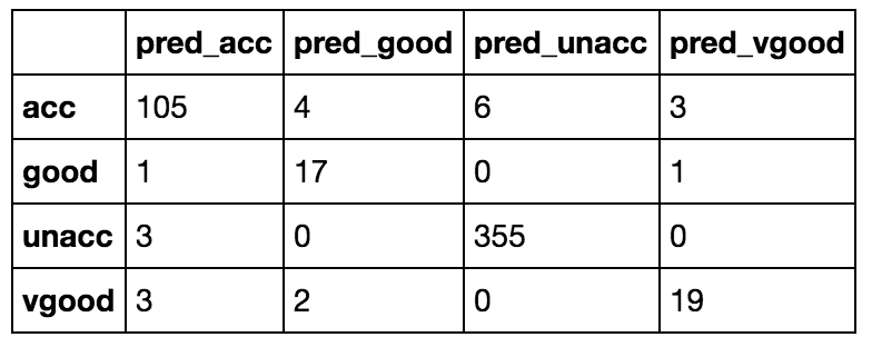
5. Loop through label enconder function classes (its classes are accurate, good, unaccurate and very good) in the following way
for c in le.classes_
6. Append all looped values with pred_as suffix so that you know they represent predicted classes
['pred_'+c for c in le.classes_]
7. Store result as a variable that will represent columns of our next DataFrame
predicted_cols = ['pred_'+c for c in le.classes_]
8. Make a DataFrame using the confusion matrix as data and the classes as index and predicted classes as columns. You will see the confusion matrix just in a different way of looking at the index and columns
pd.DataFrame(conf, index = le.classes_, columns = predicted_cols)

