What happens when your dataset is not in tabular format or features are not well defined. How do you select data features and target?
- Use Feature Selection
What’s another reason to use Feature Selection?
- to reduce computational complexity of the model
- to reduce memory footprint of dataset
- to speed up training
- to have better insight into what factors are important
- to simplify dataset
What are types of data that require Feature Selection?
- Images
- Sound
- Text
- Movies
- TimeSeries
Example of those type of data?
- To classify images, we must represent them as a vector of numbers
- To classify text data (sentence or document), we must represent them as a vector of numbers
- To classify tabular data, we must simplify it
More detailed example?
| Text | the | cat | is | on | table | blue | sky | … |
| The cat is on the table | 2 | 1 | 1 | 1 | 1 | 0 | 0 | … |
| The table is blue | 1 | 0 | 1 | 0 | 1 | 1 | 0 | … |
| The sky is blue | 1 | 0 | 1 | 0 | 0 | 0 | 1 | … |
| … | … | … | … | … | … | … | … | … |
Why for the first row, “the” column has 2 as value? (FIX!)
- Maybe because it has 0 predictive power
Tabular data example?
- Reducing number of features to simplify model while retaining predictive power, getting something like this
What are feature selection techniques?
- Bottom up feature selection
- Top Down feature selection
- Random shuffling
- Lasso and Ridge Regularization
- Feature Importance
What is Bottom up feature selection step by step?
- Find feature that gives highest score
- Iteratively add the other features one by one, checking how much score improves
- Use the following criteria: Only retain first N features that achieve 90% as good a score as all features
What is Top Down feature selection step by step?
- Impose global constraint that will force feature selection
- Global constraint: In text vectorization, impose that a feature needs word frequency higher than certain threshold
What is random shuffling step by step?
- Calculate score of a model
- Randomize values along a column from the dataset that the model is based on
- If feature has predictive power, the new score will be worse
- If feature has no predictive power, there will be no change in score. Thus, we can get rid of it
What is regularization step by step?
- Example of top-down technique for parametric models such as Logistic Regression and Support Vector Machine
- Impose global constraint (on parameters that define model) that will force feature selection
- Global constraint: Minimization of term defining model and term defining regularization
How can we express that constraint mathematically?
- In general, a regularization term
R(f)is introduced to a general loss function:
minf∑i=1nV(f(x̂ i),ŷ i)+λR(f)
Where V describes the cost of predicting f(x) when the label is y, such as the square loss or hinge loss and λ controls the importance of the regularization term. R(f) is typically a penalty on the complexity of f
How can we can express regularization term as a norm on the parameters?
As two possible parameters:
l1 or Lasso regularization:
R(f)∝∑|βi|
or
l2 or Ridge regularization:
R(f)∝∑β2i
where βi are the parameters of the model.
What is an intrinsic way of evaluating feature importance?
- Decision Trees have a way to assess how much each feature contributes to overall prediction
- In Logistic Regression, the size of each SCALED coefficient represents the impact a unit change has on the overall model
How to feature scale step by step with code?
- How to get the data?
1. Import the following packages
import pandas as pd
import numpy as np
from sklearn.linear_model import LogisticRegression
from sklearn.datasets import load_iris
2. Write load_datasetname()
load_iris()
3. Store result in a variable
iris = load_iris()
4. How to determine data features and target?
5. Identify data features and target by writing .data and .target to the variable
iris.data
iris.target
6. Store results in two variables for better manipulation
X = iris.data
y = iris.target
2. How to scale data?
- Import the following
from sklearn.preprocessing import StandardScaler
2. Write StandardScaler() function
StandardScaler()
3. Apply fit_transform to function using data features as argument (what we are fitting to scale)
StandardScaler().fit_transform(X)
4. Store result in a variable for better manipulation
X_norm = StandardScaler().fit_transform(X)
3. How to model data as a Logistic Regression Model?
- Write LogisticRegression() function
LogisticRegression()
- Store function in a variable
model = LogisticRegression()
- Model function to SCALED data features and target. Use SCALED data features and target as argument of variable.fit
model.fit(X_norm, y)

4. Notice that to specify lasso or ridge, you can set penalty parameter to either l1 or l2. Below is our current model
4. How to find the model coefficients?
1. Write variable.coef_
model.coef_
2. Use previous value as data of pandas DataFrame
pd.DataFrame(model.coef_)
3. Set columns to data features of your data set
pd.DataFrame(model.coef_, columns = iris.feature_names)
4. Set index to target of your data set
pd.DataFrame(model.coef_, columns = iris.feature_names, index =iris.target_names)5. Store results in a variable
coeffs = pd.DataFrame(model.coef_, columns = iris.feature_names, index =iris.target_names)
coeffs
5. Plot
- Import the following packages
# first import matplolib
%matplotlib inline
import matplotlib.pyplot as plt
2. Applt figure() function to plt
plt.figure()
3. Store result in a variable
fig = plt.figure()
4. Apply add_subplot(111) to variable
fig.add_subplot(111)
5. Store result in new variable
ax = fig.add_subplot(111)
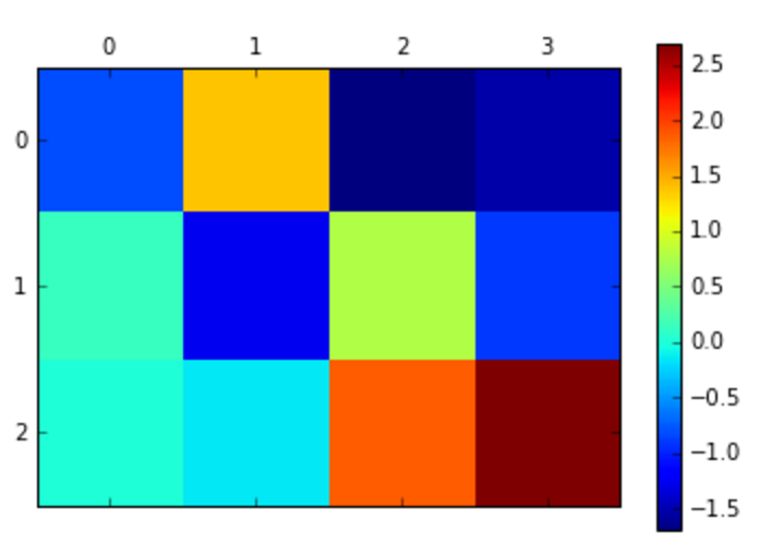
6. Apply matshow to new variable and use pandas DataFrame of coefficients as argument. For better manipulation store result in variable and see output
cax = ax.matshow(coeffs)
cax

7. Add colorbar by applying colorbar to figure function and using matshow as argument
fig.colorbar(cax)
8. Add ticks.Store DataFrame’s column values in a list and index values in another list
list(coeffs.columns)
list(coeff.index)
9. Add space list to each list so that it skips header
['']+list(coeffs.columns)
['']+list(coeff.index)
10. Use both lines as arguments of new variable (ax) dot set_xticklabels and new variable (ax) dot set_yticklabels, respectively
ax.set_xticklabels(['']+list(coeffs.columns))
ax.set_yticklabels(['']+list(coeffs.index))
11. Set rotation paremeter to your convenience
ax.set_xticklabels(['']+list(coeffs.columns), rotation=45)
ax.set_yticklabels(['']+list(coeffs.index))
6. Conclusion?
- Petal length is the most relevant length to determine setosa species
